The horizon is not your problem#
The textbook starting point for sensor height is the distance to the horizon. For a sensor at height on a sphere of radius , with refraction modeled by an effective radius ( for standard atmosphere, the convention in Skolnik):
| Height | Geometric horizon | Radar horizon (4/3 Earth) |
|---|---|---|
| 2 m | 5.05 km | 5.83 km |
| 5 m | 7.98 km | 9.21 km |
| 9 m | 10.71 km | 12.36 km |
| 15 m | 13.83 km | 15.96 km |
| 25 m | 17.85 km | 20.6 km |
| 40 m | 22.58 km | 26.06 km |
Even a 2 m post has a 5 km horizon — far beyond the size of most protected sites. On real sites the horizon is irrelevant. What limits coverage is the hill, the embankment, the warehouse, the stacked containers. That calls for a viewshed, not a formula.
Method#
We generated 30 synthetic sites (elevation_coverage.py, seed 11), each 3 × 3 km at 15 m resolution: a fractional-Brownian terrain surface (spectral exponent 3.2, scaled to 12 m standard deviation of relief) plus 0–60 rectangular buildings 8–14 m tall in the central area. For each sensor position we computed a viewshed by ray-marching 1,440 azimuths in 15 m steps and keeping the running maximum elevation angle along each ray. A ground cell at range is visible to a 1.7 m person-height target when
Experiment A put one sensor at the centre of each site at heights from 2 m to 40 m and measured visible ground within 1.2 km. Experiment B placed up to six sensors in three modes — 2 m posts, 9 m masts, and perches 2 m above the highest points including rooftops — chosen either greedily or at random.
Result A: height roughly doubles coverage from post to mast#
| Sensor height | Visible ground (mean) | Std. dev. across sites |
|---|---|---|
| 2 m | 13.9% | 12.1% |
| 5 m | 20.9% | 13.9% |
| 9 m | 28.3% | 14.6% |
| 15 m | 38.3% | 14.8% |
| 25 m | 53.4% | 14.1% |
| 40 m | 68.7% | 11.5% |
Going from a 2 m post to a 9 m mast doubles visible ground (13.9% → 28.3%). Reaching 40 m gets to 68.7%. The spread across sites is large — one standard deviation is ±12–15 points — which is the quantitative case for surveying every site rather than applying a rule of thumb.
Explore one site in 3D#
The viewer below is one synthetic site from the same generator and ray-march code (exported by viewshed_export.py, seed 23, shown at 30 m cells with vertical relief exaggerated). Sand cells are ground a standing person could be seen on from a sensor at the centre; olive cells are hidden; grey blocks are buildings; the ring is the 1.2 km analysis radius. Switch the sensor height and watch the hidden ground shrink behind each ridge — on this site visible ground goes from 5.3% at 2 m to 15.8% at 9 m and 37.4% at 25 m, a rougher site than the 30-site average above.
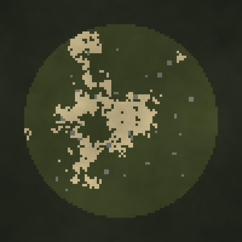
Drag to rotate · tap a height · static map shown if WebGL or motion is unavailable
Result B: placement beats height#
Maximizing the area covered by sensors is a maximum-coverage problem. The coverage function is monotone and submodular, so the simple greedy algorithm — repeatedly add the sensor with the largest marginal gain — is guaranteed to reach at least of the optimum (Fisher, Nemhauser and Wolsey, 1978). In practice it does much better than the bound.
| Sensors | 2 m post, random | 2 m post, greedy | 9 m mast, random | 9 m mast, greedy | Perch on high point, greedy |
|---|---|---|---|---|---|
| 1 | 7.4% | 23.5% | 14.9% | 34.5% | 32.3% |
| 2 | 14.0% | 36.5% | 28.4% | 53.1% | 49.6% |
| 3 | 19.8% | 45.6% | 38.4% | 64.1% | 59.7% |
| 4 | 24.9% | 51.8% | 44.7% | 71.7% | 66.8% |
| 5 | 29.2% | 56.8% | 52.4% | 77.4% | 71.8% |
| 6 | 33.2% | 60.8% | 57.3% | 81.5% | 75.4% |
Two greedily placed 9 m masts (53.1%) see about as much as six masts placed at random (57.3%). Greedy placement of six 2 m posts (60.8%) beats six randomly placed 9 m masts. If you take one number from this study: a site survey that optimizes placement is worth more than extra metres of mast.
An honest negative result#
We expected perching on the highest points to beat masts. It did not. A sentry 2 m above the best terrain and rooftop points covered 75.4% with six units against 81.5% for six greedily placed 9 m masts — consistently 2–6 points behind. On these terrains, 7 m of extra height anywhere is worth more than 2 m on the best spot.
Two caveats keep this from being the whole story. Our candidate “high points” were restricted to terrain and rooftops; light towers, pylons and crane platforms — where Kestrel perches in practice — were not modeled and would add 10–30 m. And static coverage is not what redeployability buys: a perching sentry's coverage map can be changed every hour, so the relevant comparison is against a mast that is never wrong about where the threat will come from. We will quantify that in a follow-up using adversarial path models. For now the takeaway for buyers is that height on the perch matters, and our site surveys look for tall perches first.
Running this on your own site#
The method transfers directly to a real site. Replace the synthetic surface with a digital surface model (DSM, which includes buildings and vegetation) for obstacles and a digital terrain model (DTM, bare earth) for target heights — national mapping agencies and lidar surveys publish both at 0.5–2 m resolution in many countries. The core of the viewshed is a running maximum along rays:
obst  = (dsm[ix, iy] - z0) / r          # slope to each obstacle top along every ray
horiz = np.maximum.accumulate(obst, axis=1)
prev  = np.concatenate([np.full((n_az, 1), -np.inf), horiz[:, :-1]], axis=1)
seen  = (dtm[ix, iy] + target_h - z0) / r >= prev   # target visible above everything nearer
Three practical adjustments matter on real data. Use the DSM for the observer's base height only if the sensor will actually sit on that structure. Treat vegetation as seasonal: a deciduous tree line that blocks sight in August may not in January, so run both. And restrict candidate positions to places you can actually install or perch — the greedy algorithm will happily choose the top of a chimney. Our site surveys run this with each customer's own survey data before we propose a sensor layout.
Limitations#
Synthetic terrain without vegetation; 15 m cells blur small obstacles such as walls and fences; buildings are boxes; the target is a standing person with no consideration of sensor resolution, which in reality caps useful range well inside 1.2 km for small optics (see DORI pixel density). Coverage is binary — no partial visibility, no atmospheric attenuation. Greedy placement used a pool of 80 candidates per site, not the full grid.
Frequently asked questions#
How high should a security camera tower be?
In our 30-terrain study, moving from 2 m to 9 m doubled visible ground and 40 m reached about 69%. But site-to-site variation was ±12–15 points, so survey the site.
What is the radar horizon formula?
d ≈ 4.12 √h km with h in metres, using the standard 4/3 effective Earth radius; 3.57 √h without refraction.
How do you choose where to put perimeter sensors?
Treat it as a maximum-coverage problem and place sensors greedily by marginal viewshed gain. Greedy placement is guaranteed at least 63% of optimal and in our study two greedily placed masts matched six random ones.
References#
- M. I. Skolnik, Introduction to Radar Systems, 3rd ed., McGraw-Hill. Radar horizon with the 4/3 effective Earth radius; see also MathWorks
horizonrangedocumentation. - M. L. Fisher, G. L. Nemhauser, L. A. Wolsey, “An analysis of approximations for maximizing submodular set functions,” Mathematical Programming 14 (1978), 265–294.
Reproducibility: model code is published at /research-code/ with a README. Results are model outputs under the assumptions stated above, not field trials.